Sequence Alignment Methods

Alignment strategies

The overall goal of sequence alignment is to find the best pairing of two sequences. By comparing sequences through alignment, patterns of conservation and variation can be identified. There are two main strategies that are often used: Global sequence alignment and the Local sequence alignment.

Global sequence alignment

Two sequences to be aligned are considered to be generally similar over their entire length in the global sequence alignment. Global sequence alignment is carried out between the entire length of two sequences to find the regions of the best possible alignment. This method of alignment is optimal for two closely related sequences of the same length. For the sequences that are divergent or not similar in length, global sequence alignment doesn't produce optimal results because it fails to recognize the local regions of high similarity between two sequences [1,5].

The Needleman-Wunsch algorithm is the classical global pairwise alignment algorithm employing dynamic programming [2]. Let's suppose we have two sequences; Sequence 1: ACGTGCCTTCA and Sequence 2: CATCCTTG. The global alignment between these two sequences involves the following steps; Initialization, Matrix Filling, Trace backing, Alignment. An example of a global sequence alignment between the entire length of these two sequences is discussed further.

The first step in global sequence alignment is initialization which involves the construction of a square matrix to house both sequences in rows and columns. There are some important rules to consider before proceeding to matrix filling. At the starting of the matrix extra row and column is given for adding gaps. Once the scoring matrix is created the gap, match and mismatch scores are arbitrarily assigned by the user, and they do not have to be specific. The first column and row starting from 0 are filled by adding the gap scores in each previous block (Figure 1).

The alignment scoring starts by adding the scores from left, bottom and diagonal box and choosing the highest value to put in that box. If the value is coming from the left box the gap score is added, if the value is coming from the bottom box, the gap score is added, but if the value is coming from the diagonal box, we add match or mismatch score depending on our sequence. For this example, the scoring scheme is; Gap score: -2, Match score: +5 and Mis-match score: -1. For filling the matrix, the scores from left, bottom and diagonal blocks are considered. As mentioned previously, if the scores are coming from left or bottom blocks the gap score is added into the scores of left and bottom blocks. If the score is coming from the diagonal block, the match or mismatch score is added. If two nucleotide sequences match, the match score is added into the score of the diagonal block and vice versa (Figure 2).

The two sequences are scored at their entire length and the block from which the highest score is obtained is marked to ease trace backing, which is the third step in the global sequence alignment algorithm. When all the cells are filled with scores, the best alignment is determined through a trace-back procedure to search for the path with the best total score. For backtracking, start from the top box of the matrix towards the origin of the matrix. When a path moves horizontally or vertically, a penalty is applied. The best matching path is the one with the maximum score (Figure 3).

Local sequence alignment

The divergence level between the two sequences to be aligned is not easily recognized in the regular sequence alignment. The sequence length of two sequences can sometimes be unequal, and in such case, it is preferred to find the regions of local similarity than to scan to the whole length of two sequences. The Smith-Waterman algorithm is the first algorithm to employ dynamic programming for local sequence alignment [3]. In this algorithm, positive scores are given to the matches and zeros to the mismatches. No negative scores are used in this algorithm. Local sequence alignment is suitable to align divergent sequences at the cost of full-length alignment, but it finds the best local regions of similarity between two sequences of different origin [1,6].

The local sequence alignment involves the same overall steps as the global sequence alignment. Initialization, matrix filling, trace backing and alignment. Same two above sequences are used in the following example of local alignment as the global sequence alignment and the scoring scheme used in this example of local sequence alignment is: Gap score: -2, Match score: +1 and Mismatch score: -1.

The matrix initialization begins with assigning both sequences in rows and columns with a gap before each just like global sequence alignment. Gap scores are added to fill the first row and column of the square matrix since negative scores are not allowed in local alignment algorithm; the first row and column is just zeros (Figure 4). The next step in local sequence alignment is matrix filling. The rules of matrix filling are the same as the global sequence alignment, i.e., if the scores are coming from left or bottom blocks, the gap score is added into the scores of left and bottom blocks. If the score is coming from the diagonal block, the match or mismatch score is added. If two nucleotide sequences match, the match score is added into the score of the diagonal block and vice versa. The only difference is the negative scores cannot be added into the matric (Figure 5).

After filling the matrix, the next step in local sequence alignment i trace backing. The matrix is traced back from the top to the origin of the matrix to find regions of best scores. The best matching path is the one that has the maximum total score. If two or more paths reach the same highest score, then one is chosen arbitrarily to represents the best alignment. The path can also move horizontally or vertically at a certain point (in case, if the highest score of cells comes from left or bottom cell's score), which corresponds to the introduction of gap or an insertion or deletion for one of the two sequences. In local alignment, we only trace back local (fully aligned region without mismatch or gaps) aligned region. The traced back regions are aligned in the last step (Figure 6).

Phylogenetic tree construction methods

Phylogenetics is the study of the evolutionary relationship between organisms using a tree like diagram. The tree branching pattern represents evolutionary relationships between organisms. There are two main methods for phylogenetic tree construction, Distance-Based Methods and Character-Based Methods [7,8]. These methods are further sub-divided into different categories.

Distance-Based Methods

Phylogenetic trees can be constructed using the distance-based method, which relies explicitly on the genetic distances between sequences. This method requires the sequence data to be transformed into a pairwise similarity matrix for use during tree inference. The distance-based algorithm can be further sub-divided into the clustering-type algorithms and the optimality-based algorithms. The clustering-type algorithms construct trees starting from most similar sequence pairs. They include the unweighted pair group method using arithmetic average (UPGMA) and neighbor-joining (NJ). The optimality-based algorithms compare different tree topologies and select the one that best fits the actual evolutionary distance [1,9-12]. These include Fitch-Margoliash method and the Minimum Evolution method.

Unweighted Pair Group Method Using Arithmetic Average (UPGMA)

Unweighted Pair Group Method Using Arithmetic Average method constructs a rooted phylogenetic tree (dendrogram) using distance matrix obtained from the alignment of different sequences. UPGMA assume that all taxa evolve at a constant rate, however real data rarely meet this assumption [10].

Starting from a distance matrix, two taxa with the smallest pairwise distance are paired. The new pair is treated as a single taxon and the distance between the new taxon and all remaining taxa is calculated to form a reduced matrix. The process is repeated until no further taxa are left. An example of phylogenetic tree construction using the UPGMA algorithm is discussed below.

Consider the four different sequences; Sequence A: AACTGGCTTA, Sequence B: AACTCGGTTA. Sequence C: CATTGGCATA and Sequence D: CCCTGAAACC. Align these sequences to find the mismatched regions (Figure 8).

A distance matrix is constructed using the MSA data; by using this distance matrix, the UPGMA algorithm starts grouping two taxa with the shortest distance. After grouping, those taxa will consider as a single taxon. A node is placed at the midpoint of those taxa (Figure 9). The distance between this new composite taxon and all next taxa is again calculated, and then the taxon which is at the shortest distance from composite taxon is grouped with it. The same grouping process is repeated and another newly reduced matrix is created. The process continues until all taxa are placed on the tree. Outgroup of tree is the last taxon that is added in the end of the process, producing a rooted tree. In this method, all taxa evolve at a constant rate, and they are equally distant from the root (real data rarely meet this assumption). UPGMA often produces erroneous tree topologies. However, owing to its fast speed of calculation, it has found extensive usage in clustering analysis of DNA sequence data.

As taxon A and B are at the shortest distance, A-B is combined and treated as a single taxon. In the UPGMA method, all taxa are at equidistant from the node thus branch length of A and B from the node is given as AB/2 = 2/2 = 1; as a result, new composite taxon A-B is created (Figure 9). After those new distances are calculated to construct a reduced matrix. The total distance of C from A and C from B are summed up and divided by 2 to get the new distance of C from A-B. Similarly, the distance of D from A-B is calculated. The taxon with the smallest distance is picked again from this newly constructed distance matrix and added to the tree (Figure 10).

As taxon C is equidistant from taxon AB (AB-C/2 = 4/2 = 2). The distance of D is calculated from A-B-C and since D is at equidistance from taxon A-B-C (ABC-D/2 = 7/2 = 3.5) and the final outgroup is placed (Figure 11).

Neighbor-Joining Method

Neighbor-joining is a standard way of constructing a phylogenetic tree. It is somewhat similar to the UPGMA method in that it builds tree step-wise starting from the shortest distance and moving towards the longest distance step by step. NJ method also uses a reduced matrix for tree construction. However, this method does not assume all the taxa to be equidistant from the root; it calculates actual evolutionary rates or distance between sequences [1,11]. This method uses the conversion step to calculate the actual distance of taxa from their root, using the following formula:

d’AB = dAB – 1/2 (rA + rB) ……(Eq. i)

Whereas d'AB is the converted distance between A and B, dAB is the actual evolutionary distance between A and B and rA (or rB) is the sum of distances of A from all other taxa. The r-value (for example, rA) can be calculated using equation ii. The r-values are used to construct a reduced matrix.

rA = ∑dAB ……(Eq. ii)

A and B in equation ii represents two different taxa. The transformed r-value (r') is required to calculate the distance of an individual taxon from its node.

r’A = rA/n-2 ……(Eq. iii)

Where n is the total number of taxa. Let's assume A and B form a node called U, the distance of individual taxa (taxa A or B) from the node U can be calculated using the following equation:

dAU = [dAB + (r’A – r’B)] /2 ……(Eq. iv)

In the NJ method, before the construction of the tree, all the given taxa are collapsed into a star tree. Then the pair of taxa having the shortest distance in the matrix is separated from the star and built into a single composite taxon with a node. After the first node is constructed, the newly created taxon is considered as a single taxon, allowing the next most closely related taxon to be joined next to the first node which will create the second node for a new taxon. The cycle is iterated until all internal nodes are resolved. This whole process is also known as star decomposition because it starts with the star formation and decomposition of that star into a tree diagram based on the distances between taxa. NJ method produces an unrooted tree; outgroups are determined on the basis of external knowledge.

Consider the following example of tree construction using the Neighbor-Joining method. For this example, the same pairwise distance matrix given in Figure 9 is used. The first step in the NJ method is the calculation of r and r' value using equation ii and iii.

The r-value is calculated as:

rA = AB+AC+AD = 2+3+7 = 12, rB = BA+BC+BD = 2+5+8 = 15,

rC = CA+CB+CD = 3+5+6 = 14, rD = DA+DB+DC = 7+8+6 = 2

The r' value is calculated as:

r’A = rA/n-2 = 12/4-2 = 12/2 = 6, r’B = rB/n-2 = 15/4-2 = 15/2 = 7.5

r’C = rC/n-2 = 14/4-2 = 14/2 = 7, r’D = rD/n-2 = 21/4-2 = 21/2 = 10.5

The corrected distances are calculated using equation i to create a new distance matrix (Figure 12) as:

d’AB = 2 – 1/2*(12 + 15) = 2 – 27/2 = 2 – 13.5 = –11.5

d’AC = 3 – 1/2*(12 + 14) = 3 – 26/2 = 3 – 13 = –10

d’AD = 7 – 1/2*(12+21) = 7 – 33/2 = 7 – 16.5 = –9.5

d’BC = 5 – 1/2*(15 + 14) = 5 – 29/2 = 5 – 14.5 = –9.5

d’BD = 8 – 1/2*(15 + 21) = 8 – 36/2 = 8 – 18 = –10

d’CD = 6 – 1/2*(14 + 21) = 6 – 35/2 = 6 – 17.5 = –11.5

The next step in the NJ method is the grouping of taxa, before this, all possible nodes are collapsed to form a star, then the taxa get separated step by step from this star diagram according to their distances (this is why the NJ method is also known as star deformation). According to the distance matrix in Figure 12, A and B taxa are at shortest distance, so these taxa are separated from the star and are grouped together to form a single composite taxon with a node "U" in the middle of both taxon (Figure 13).

The branch length of A and B to the node U is calculated using equation iv as:

dAU = [2 + (6 – 7.5)]/2 = [2 + (–1.5)]/2 = 0.5/2 = 0.25

dBU = [2 + (7.5 – 6)]/2 = [2 + 1.5]/2 = 3.5/2 = 1.7

The branch lengths on the NJ phylogenetic tree are adjusted taking into account the new branch length distances (Figure 14).

New composite taxon allows the construction of reduce matrix. Start with actual distances and again construct distance matrix for other taxa (C, D).

dCU = [(dAC – dUA) + (dBC – dUB)]/2 = dCU = [(3 – 0.25) + (5 – 1.75)]/2 = [2.75 + 3.25]/2 = 6/2 = 3

dDU = [(dAD – dUA) + (dBD – dUB)]/2 = dDU = [(7 – 0.25) + (8 – 1.75)]/2 = [6.75 + 6.25]/2 = 13/2 = 6.5

The new r-values and the r’-values are calculated using the new composite distance matrix (Figure 15). The corrected distances are calculated using this distance matrix and a new distance matrix with correct evolutionary distances between taxa is obtained (Figure 15).

According to figure 15, the taxon C have the shortest distance to node U. So, the taxon C is grouped with A-B (it creates new composite taxon A-B-C). A new node "V" is created from U to C. Before grouping of the taxa, the branch lengths are first calculated (Figure 16).

dCV = [3 + (9 – 9.5)]/2 = [3 + (–0.5)]/2 = 2.5/2 = 1.25

dDV = [3 + (9.5 – 9)]/2 = [3 + 0.5}/2 = 3.5/2 = 1.75

Optimality-Based Methods

Clustering-based algorithms only produce a single tree as an outcome. However, it is not possible to determine how this tree is compared with other alternate trees. The optimality-based method has a well-defined algorithm which compares all possible tree topologies and selects a tree that best fits the evolutionary distance matrix. This method is exhaustive and has slow computation. There are two types of algorithms in optimality-based method Fitch–Margoliash (FM), Minimum Evolution (ME) [13,14].

Fitch-Margoliash

The Fitch-Margoliash approach selects the best tree among all available trees based on the minimal deviation between the distances calculated in the overall branches in the tree and the distances in the original dataset. It starts by clustering two taxa with the shortest distance in a single node and temporarily combining all other taxa into a group (Figure 17). It then creates an unrooted 3 taxa tree. Three algebraic equations are solved to determine the branch lengths and distances. The clustering to two taxa helps create a new reduced matrix, and this process is iterated until the tree is entirely resolved. This method selects the best tree among all tree topologies that has the lowest squared deviation of actual distances and calculated tree branch lengths [15]. The criterion of optimality is described by the following formula: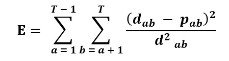

Where E is the error of the estimated tree fitting the original data, T is the number of taxa, dab is the pairwise distance between A and B taxa in the original dataset, and pab is the corresponding tree branch length [1].

The distances are calculated using the following algebraic equations:

dAB = a + b

dAC = a + c

dBC = b + c

The branch lengths are calculated using the following equations:

a = (dAB + dAC – dBC)/2

b = (dAB + dBC – dAC)/2

c = (dAC + dBC – dAB)/2

Consider the following example of tree construction using the Fitch-Margoliash algorithm; The tree construction starts by constructing a distance matrix by calculating dissimilarities between sequences just like done in previous examples. Two taxa with the smallest distance are clustered together in a single node, and all other taxa are temporarily combined into a single group.

Since we combined taxa C, D and E into a single group we need to find the distance of taxa A and B to C-D-E (Figure 19) in order to calculate the branch lengths.

dA-CDE = [(dAC) + (dAD) + (dAE)]/3 = 7 + 11 + 12/3 = 30/3 = 10

dB-CDE = [(dBC) + (dBD) + (dBE)]/3 = 9 + 10 + 10/3 = 29/3 = 9.667

Now using the newly created reduced distance matrix the branch lengths are calculated as follow:

a = (dAB + dA-CDE – dB-CDE)/2 = 2 + 10 – 9.667/2 = 2.333/2 = 1.1665

b = (dAB + dB-CDE – dA-CDE)/2 = 2 + 9.667 -10/2 = 1.667/2 = 0.8335

cde = (dA-CDE + dB-CDE – dAB)/2 = 10 + 9.667 – 2/2 = 17.667/2 = 8.8335

Now we can treat taxa A and B as a single group and separate C-D-E to create a new distance matrix (Figure 21). The taxa with the shortest distance are selected again from the matrix and their branch length is calculated.

Taxa D-E are at the shortest distance in the new distance matrix, so they are clustered in a single node and all other taxa are grouped together (A-B-C). The distance of D and E to the newly created group is calculated as follow:

dD-ABC = [(dAD)+(dBD) +(dCD)]/3 = 11+10+5/3 = 26/3 = 8.667

dE-ABC = [(dAE)+(dBE) +(dCE)]/3 = 12+10+5/3 = 27/3 = 9

Only the C taxon is left so to calculate its branch length taxa A-B and D-E are combined to create a new reduced matrix (Figure 24).

The branch length is calculated using the new distances obtained in reduced matrix.

ab = (dAB-C + dAB-DE – dC-DE)/2 = 8+10–5/2 = 13.75/2 = 6.875

c = (dAB-C + dDE-C – dAB-DE)/2 = 8+5–10.75/2 = 2.25/2 = 1.125

de = (dAB-DE + dDE-C – dAB-C)/2 = 10.75+5-8/2 = 7.75/2 = 3.875

The final step is to join all the branches into a single tree. We obtained three trees, so they are joined together to form a single tree (Figure 26).

Now to calculate the branch length of a in figure 26 subtract the average of A and B (A+B/2 = 1.1665+0.8335/2 = 2/2 = 1) from the branch length of AB (a = [(AB) – (A+B/2)] = 6.875 – 1 = 5.875). Similarly, for b the average of D and E (D+E/2 = 1.8335+2.1665/2 = 4/2 = 2) is subtracted from branch length DE (b = [(DE) – (D+E/2)] = 3.875 – 2 = 1.875). Adding these final branch lengths, a complete phylogenetic tree with correct evolutionary distances is obtained (Figure 27).

Minimum Evolution

Minimum evolution constructs a tree with a similar method but uses a different criterion of optimality that finds a tree with a minimum total branch length among all possible trees. The following formula describes the criterion of optimality:

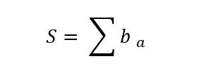
Where S is the sum of branch lengths for given tree topologies and ba is the ath branch length. The theoretical basis of the minimum evolution method is the statistical evidence presented by A. Rzhetsky and M. Nei in 1993 [16] that shows that when unbiased estimates of evolutionary distances are used, regardless of the number of sequences, the predicted value of S becomes smaller for true topology.

Character-Based Methods

The character-based methods compare all sequences simultaneously considering one character/site at a time. Character-based methods include maximum parsimony and maximum likelihood. These approaches use probability and take into account the sequence variations [17]. Both methods take the tree with the highest score into consideration, which needs a minimum number of changes to align.

Maximum Parsimony

Maximum Parsimony (MP) is the most common and widely accepted tree construction approach to date [18]. Because it uses a character-based algorithm, this approach is different from the distance-based approaches previously discussed. This approach works by scanning through all potential tree structures and assigning a cost to each tree. Parsimony is based on the presumption that the most possible tree is the one that needs the least number of changes to explain the alignment data [19]. The premise that taxa or nodes are sharing a common characteristic does so because it inherited that attribute from a common ancestor [20].

Conflicts with this approach are explained under the term homoplasy. There are three ways of reserving conflicts: reversal (return to the original state), convergence (unrelated taxa evolved the same characteristic completely independently) and parallelism (different taxa may have similar mechanisms that develop a character in a certain way) [19,20]. The tree with a lowest tree score or length, as determined by the number of changes accumulated along the branches, is called the most parsimonious tree, and it best represents the evolutionary pattern [20,21].

Maximum Parsimony is also different from other approaches as it does not find the branch lengths but the total overall length in terms of the number of changes.

Maximum Parsimony often considers two or more trees equal and provides no direct answer on which tree is the actual evolutionary tree. A strict (majority rule) consensus is used to overcome this problem in most situations.

Traditional Parsimony method uses recursion to find the minimum amount of change within the trees. This is done by starting at the leaf of a tree and working up towards the root. It is known as post-order transversal [18,20]. Whereas the other approach, Weighted Parsimony, gives the algorithm a cost factor and weights certain scenarios accordingly.

Often an artefact known as the Long-Branch Attraction exists in parsimony approach, and it should be handled. The length of the branch shows the number of substitutions between taxa or nodes. Parsimony assumes that all taxa evolve at the same rate and contribute that same amount of information [20]. Long-branch is the phenomena in which rapidly evolving taxa are grouped together on a tree when they have numerous mutations (Figure 28). Anytime two long branches are present, they may be attracted to one another [20].

Maximum Likelihood

Maximum Likelihood method was proposed by Felsenstein in 1981 [22]. This is one of the most computationally intensive methods, but it is most flexible. ML uses probabilistic models to choose a best tree that has the highest probability or likelihood of reproducing the observed data [1]. ML trees represent the most accurate evolutionary processes. This approach considers every single position in the alignment data to search for all possible tree topologies and not only the informative sites. ML calculates the total probability of ancestral sequences evolving to internal nodes and ultimately to current sequences by using a specific substitution model that has probability values of residue substitutions. For instance, for DNA sequences using the Jukes-Cantor model, the probability (P) that a nucleotide remains the same after the time (t) is:

                           P(t) = 1/4 + 3/4e-αt

Where α is the nucleotide substitution rate which is either empirically allocated or calculated from the raw

datasets. The ability to render statistical associations between topologies and data sets is one of ML's major advantages. Maximum Likelihood makes predictions. that the model used is accurate and that the approach is inconsistent if the model does not correctly represent the underlying data set. A downside of ML is the rigorous computation, and recent research indicates that a given phylogenetic tree may have multiple maximal probability points [23] (Table 1).

References

- Xiong J Essential bioinformatics. Chapter: Book Name. 2006 of publication; Cambridge University Press.
- Needleman SB, Wunsch CD. A general method applicable to the search for similarities in the amino acid sequence of two proteins. Journal of molecular biology, (1970); 48(3): 443-453.
- Smith TF, Waterman MS. Comparison of biosequences. Advances in applied mathematics, (1981); 2(4): 482-489.
- Hanmandlu M, Sani A, Gaur D. Modified k-Tuple method for the construction of phylogenetic trees. Trends in Bioinformatics, (2015); 8(3): 75.
- Huang X. On global sequence alignment. Bioinformatics, (1994); 10(3): 227-235.
- Rognes T (2011) Determination of optimal local sequence alignment similarity score. Google Patents.
- Hu Y-C, Tiwari S, Mishra KK, Trivedi MC, Munjal G, et al. Phylogenetics Algorithms and Applications. Ambient Communications and Computer SystemsRACCCS-2018, (2018); 904187-194.
- Burr T. Phylogenetic trees in bioinformatics. Current Bioinformatics, (2010); 5(1): 40-52.
- Bruno WJ, Socci ND, Halpern AL. Weighted neighbor joining: a likelihood-based approach to distance-based phylogeny reconstruction. Molecular biology and evolution, (2000); 17(1): 189-197.
- Stefan Van Dongen T, Winnepenninckx B. Multiple UPGMA and neighbor-joining trees and the performance of some computer packages. Mol Biol Evol, (1996); 13(2): 309-313.
- Saitou N, Nei M. The neighbor-joining method: a new method for reconstructing phylogenetic trees. Molecular biology and evolution, (1987); 4(4): 406-425.
- Moret BM, Warnow T (2002) Reconstructing optimal phylogenetic trees: A challenge in experimental algorithmics. Experimental Algorithmics: Springer. pp. 163-180.
- Hillis DM. Approaches for assessing phylogenetic accuracy. Systematic Biology, (1995); 44(1): 3-16.
- Saitou N, Imanishi T. Relative efficiencies of the Fitch-Margoliash, maximum-parsimony, maximum-likelihood, minimum-evolution, and neighbor-joining methods of phylogenetic tree construction in obtaining the correct tree. (1989).
- Peng C. Distance based methods in phylogenetic tree construction. NEURAL PARALLEL AND SCIENTIFIC COMPUTATIIONS, (2007); 15(4): 547.
- Desper R, Gascuel O. Theoretical foundation of the balanced minimum evolution method of phylogenetic inference and its relationship to weighted least-squares tree fitting. Molecular Biology and Evolution, (2004); 21(3): 587-598.
- Alon N, Chor B, Pardi F, Rapoport A. Approximate maximum parsimony and ancestral maximum likelihood. IEEE/ACM Transactions on Computational Biology and Bioinformatics, (2008); 7(1): 183-187.
- Durbin R, Eddy SR, Krogh A, Mitchison G Biological sequence analysis: probabilistic models of proteins and nucleic acids. Chapter: Book Name. 1998 of publication; Cambridge university press.
- Hall BG Phylogenetic trees made easy: A how to manual. Chapter: Book Name. 2011 of publication; Sinauer.
- Rizzo J, Rouchka EC. Review of phylogenetic tree construction. University of Louisville Bioinformatics Laboratory Technical Report Series, (2007); 2-7.
- Sharma A, Jaloree S, Thakur RS. Review of Clustering Methods: Toward Phylogenetic Tree Constructions; 2018. Springer. pp. 475-480.
- Felsenstein J. Evolutionary trees from DNA sequences: a maximum likelihood approach. Journal of molecular evolution, (1981); 17(6): 368-376.
- Dorigo M, Di Caro G. Ant colony optimization: a new meta-heuristic; 1999. IEEE. pp. 1470-1477.
This work is licensed under a Creative Commons Attribution-Non Commercial 4.0 International License. To read the copy of this license please visit: https://creativecommons.org/licenses/by-nc/4.0